Assignment One Report

Datasets we Picked

(Categorical) Mushroom

• Source: UCI Machine Learning Repository (ID: 73).
• Dataset Size: 5,644 samples (after dropping missing values). The test split contains 1,694 samples.
• Number of Features: 22 categorical features (e.g., cap-shape, odor, habitat).
• Class Distribution: Approximately 62% Edible (Class 0: 1058 samples in test) and 38% Poisonous (Class 1: 636 samples in test).

(Numerical) Credit Card Fraud Detection 2023

• Source: Kaggle (nelgiriyewithana/credit-card-fraud-detection-dataset-2023).
• Dataset Size: 568,630 samples. The test split contains 113,726 samples.
• Number of Features: 29 numerical features (V1 through V28, plus Amount).
• Class Distribution: Perfectly balanced. 50% Legitimate (Class 0: 56,750 samples in test) and 50% Fraudulent (Class 1: 56,976 samples in test).

---

Principal Component Analysis (PCA)

The PCA algorithm was implemented from scratch using standard linear algebra operations to change the original basis vectors of the training examples into better ones.

How it was done

1. Mean Centering
   • $X_{centered}=X-\mu$
   • What it does?
     • Shifts the dataset so that the origin $(0,0)$ is the center of the data. This is what makes the $\frac{1}{n\_samples-1}\cdot (X_{centered}^T\cdot X_{centered})$ evaluate to the covariance matrix.
2. Covariance Matrix calcualtion
   • $\Sigma =\frac{1}{n\_samples-1}\cdot (X_{centered}^T\cdot X_{centered})$
   • What it does?
     • Computes the covariance between all pairs of features, that is how they “move” together.
3. Eigenvectors calculation
   • Evals, EVs = np.linalg.eigh(cov)
   • What it does?
     • It extracts the Eigenvectors of the cov matrix, which are the directions of max. variance, and the eigen value of each one (that is the mag. of its variance)
     • Each eigen vector is a column in EVs, and they have the same index as their eigen value in Evals.
4. Finding the top eigen vectors
   • Sort EVs descending, via Evals, and the keep top $k$.
   • What it does?
     • keeps the k top eigen vectors in variance, and declare them as the new axes for the dataset. ($C_{old}$ → old identity components | $C_{new}$ → new principal components)
5. Changing the Axes of the dataset
   • _$X_{PCA}=X_{centered}\cdot C_{new}$ (done in transform)
   • What it does?
     • changes the basis vectors of $X$ from the identity ones to the new principal components $C_{new}$

---

Results and Comparison

Performance Table

Dataset	Baseline (All Features)	Feature Selection (k=10)	PCA (From Scratch)
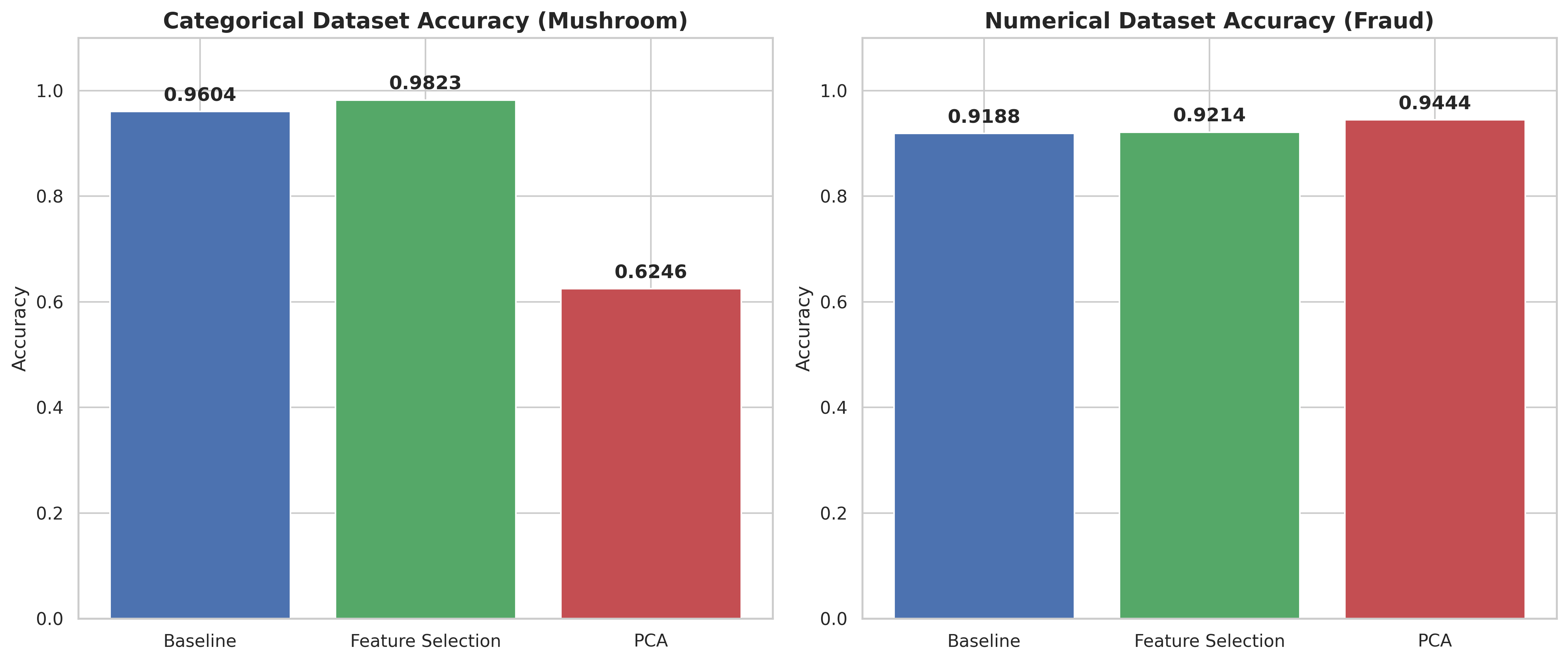
Categorical (Mushroom)	96.04%	98.23%	62.46% (at $k=1$)
Numerical (Credit Card)	91.88%	92.14%	94.44% (at $k=20$)

Questions

How did Naive Bayes perform on categorical vs. numerical data?

Categorical NB excelled (96.04% baseline), because frequency counting naturally fits discrete data. Gaussian NB performed well (91.88%) but was slightly less precise, likely due to features not perfectly following a normal distribution.

Which approach achieved the best results?

• Categorical (Mushroom): Feature Selection (98.23%). Removing redundant categories allowed for cleaner probability calculations.
• Numerical (Credit Card): PCA (94.44%). Distilling 29 features into 20 orthogonal variables satisfied the “independent feature” assumption of Naive Bayes, boosting accuracy.

How did these compare to the baseline?

Numerical results improved with both Feature Selection (+0.26%) and PCA (+2.56%). Categorical results improved with Feature Selection (+2.19%) but crashed with PCA (-33.58%).

What are the trade-offs between Selection and Reduction?

• Feature Selection: Keeps original features for high interpretability but discards data from omitted columns.
• PCA (Reduction): Preserves information from all features via compression but destroys interpretability by creating mathematical abstractions.

Is PCA appropriate for categorical data?

Absolutely not. PCA relies on Euclidean distances; since categories like “Red” or “Blue” have no meaningful numerical distance, calculating their variance results in mathematical nonsense, proven by the massive accuracy drop.

---

Visualizations

Accuracy bar charts

(for each dataset type)

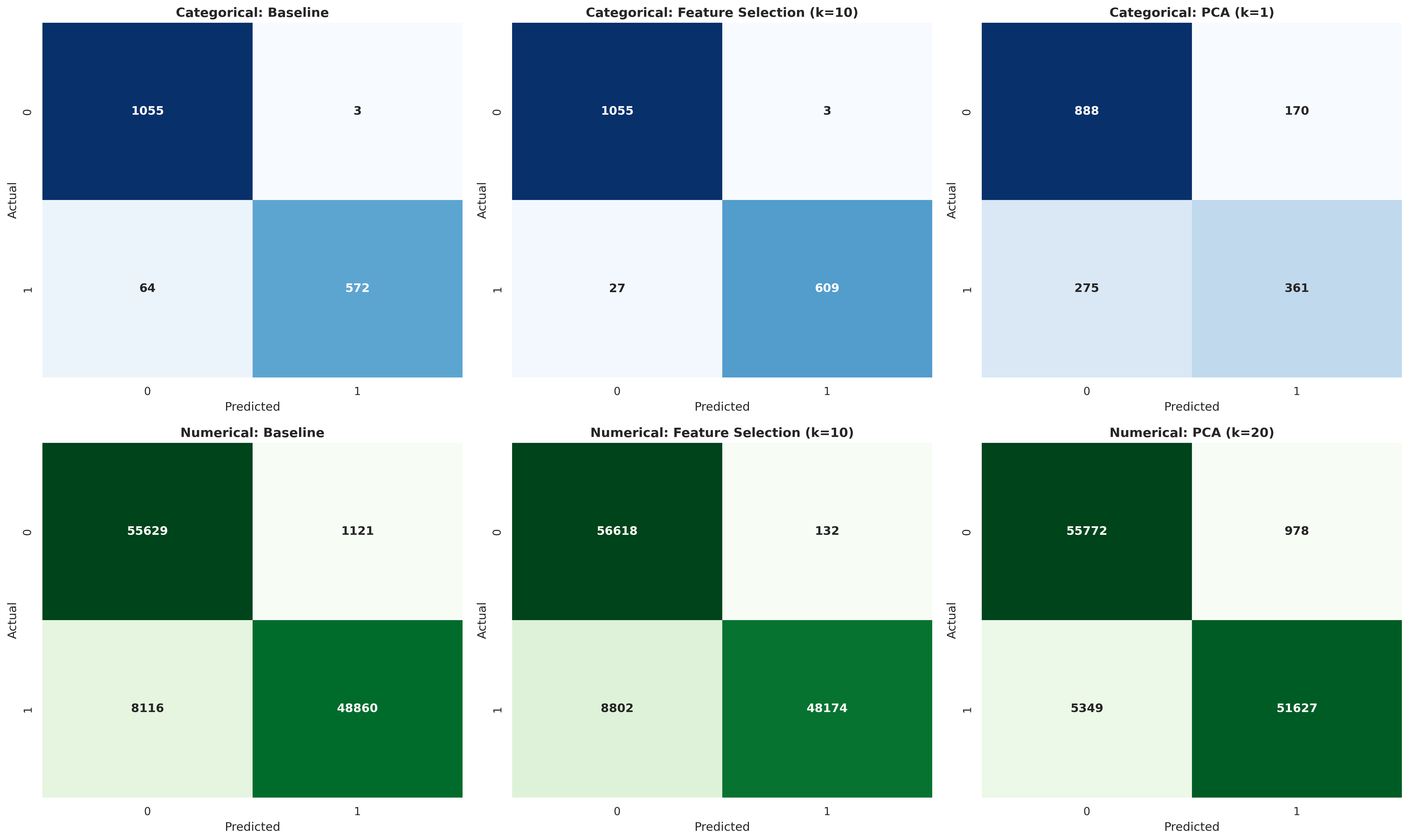
Confusion matrices

(for each experiment on each dataset type)

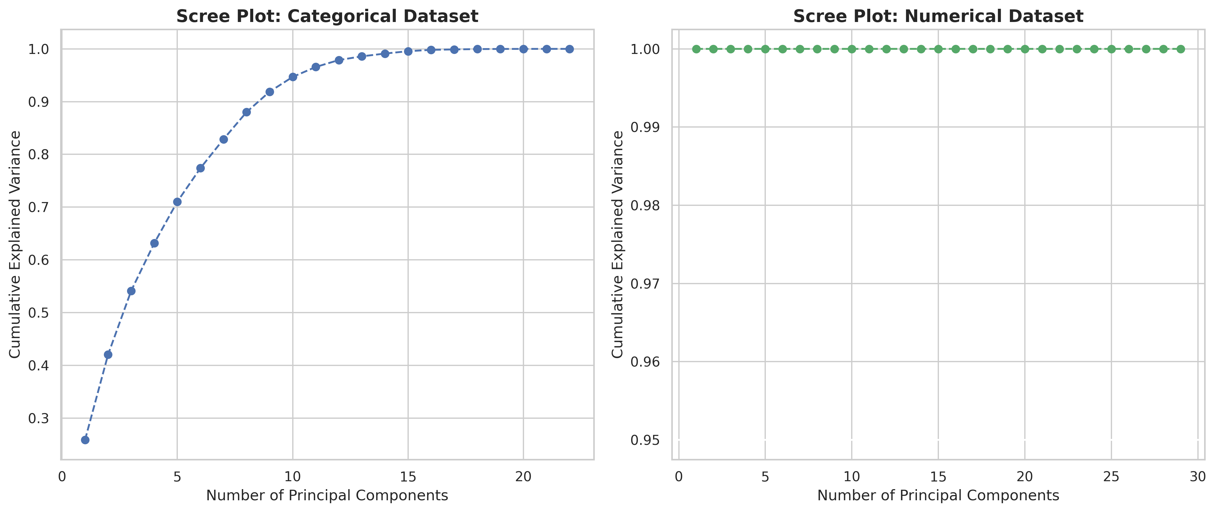
Scree plots

(for each dataset type in the experiment B)